asymptote draw 3d circles in space

Other versions of asymptote

[ < ]

[ > ]

[ << ]

[ Upwards ]

[ >> ]

[Top]

[Contents]

[Index]

[ ? ]

---

7.27 three

This module fully extends the notion of guides and paths in Asymptote to iii dimensions. It introduces the new types guide3, path3, and surface. Guides in 3 dimensions are specified with the same syntax equally in two dimensions except that triples (ten,y,z) are used in identify of pairs (ten,y) for the nodes and management specifiers. This generalization of John Hobby's spline algorithm is shape-invariant under three-dimensional rotation, scaling, and shifting, and reduces in the planar case to the two-dimensional algorithm used in Asymptote, MetaPost, and MetaFont [cf. J. C. Bowman, Proceedings in Applied Mathematics and Mechanics, 7:ane, 2010021-2010022 (2007)].

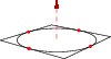
For example, a unit circle in the XY plane may be filled and drawn like this:

import three;  size(100);  path3 k=(i,0,0)..(0,one,0)..(-i,0,0)..(0,-1,0)..cycle; depict(g); draw(O--Z,red+dashed,Arrow3); depict(((-i,-1,0)--(1,-one,0)--(i,1,0)--(-1,1,0)--wheel)); dot(g,red);        

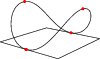
and so distorted into a saddle:

import three;  size(100,0); path3 g=(1,0,0)..(0,ane,1)..(-1,0,0)..(0,-1,1)..cycle; draw(1000); draw(((-1,-1,0)--(1,-1,0)--(ane,1,0)--(-i,1,0)--bike)); dot(g,reddish);        

Module iii provides constructors for converting two-dimensional paths to three-dimensional ones, and vice-versa:

path3 path3(path p, triple plane(pair)=XYplane); path path(path3 p, pair P(triple)=xypart);        

A Bezier surface, the natural ii-dimensional generalization of Bezier curves, is defined in three_surface.asy as a structure containing an array of Bezier patches. Surfaces may drawn with ane of the routines

void describe(movie pic=currentpicture, surface s, int nu=i, int nv=1,           material surfacepen=currentpen, pen meshpen=nullpen,           light light=currentlight, lite meshlight=low-cal); void draw(picture picture show=currentpicture, surface due south, int nu=ane, int nv=one,           material[] surfacepen, pen meshpen,           light light=currentlight, light meshlight=light); void draw(picture flick=currentpicture, surface s, int nu=one, int nv=1,           cloth[] surfacepen, pen[] meshpen=nullpens,           low-cal light=currentlight, light meshlight=light);        

The parameters nu and nv specify the number of subdivisions for drawing optional mesh lines for each Bezier patch. Here material is a construction divers in three_light.asy:

struct textile {   pen[] p; // diffusepen,ambientpen,emissivepen,specularpen   real opacity;   real shininess;     real granularity; ... }        

These material properties are used to implement OpenGL-style lighting, based on the Phong-Blinn specular model. Sample Bezier surfaces are contained in the case files BezierSurface.asy, teapot.asy, and parametricsurface.asy.

The examples elevation.asy and sphericalharmonic.asy illustrate how to depict a surface with patch-dependent colors. The examples vertexshading and smoothelevation illustrate vertex-dependent colors, which is supported for both the OpenGL renderer and two-dimensional projections. Since the PRC output format does not support vertex shading of Bezier surfaces, PRC patches are shaded with the mean of the four vertex colors.

There is no fill control for arbitrary three-dimensional cyclic paths (this would be an ill-posed operation). However, a surface constructed from a convex path3 with the constructor

surface surface(path3 external, triple[] internal=new triple[],                 triple[] normals=new triple[], pen[] colors=new pen[]);        

and then filled:

draw(surface(path3(polygon(5))),scarlet); draw(surface(unitcircle3),red); draw(surface(unitcircle3,new pen[] {cherry,greenish,blue,black}));        

The last example constructs a patch with vertex-specific colors.

Alternatively, a 3-dimensional planar path constructed from a two-dimensional (mayhap nonconvex) cyclic and nonselfintersecting path p can be filled by get-go using Orest Shardt's bezulate routine to decompose p into an array of circadian paths of length 4 or less. This array tin then be used to construct and draw a planar surface:

draw(surface(bezulate((0,0)--East+2N--2E--E+N..0.2E..cycle)),red);        

The routine surface planar(path3 p) uses bezulate to convert a three-dimensional planar (possibly nonconvex) cyclic and nonselfintersecting path to a surface.

Arbitrary thick 3-dimensional curves and line caps (which the OpenGL standard does not require implementations to provide) are synthetic with the routine

surface tube(path3 one thousand, existent width);        

which returns a tube of diameter width centered on g. This can make files slow to render, particularly with the Adobe Reader renderer. The setting thick=simulated can be used to disable this feature and force all lines to be drawn with linewidth(0) (1 pixel wide, regardless of the resolution). Past default mesh and contour lines in 3-dimensions are always drawn thin, unless an explicit linewidth is given in the pen parameter or the setting thin is set to simulated. The pens sparse() and thick() defined in plain_pens.asy can likewise be used to override these defaults for specific draw commands.

In that location are four choices for viewing 3D Asymptote output:

2. Apply the default Asymptote adaptive OpenGL-based renderer (with the command-line option -V and the default settings outformat="" and render=-ane). If you run into warnings from your graphics card driver, attempt specifying -glOptions=-indirect on the command line. On UNIX systems, we recommend installing a patched version of the freeglut library to support antialiasing via multisampling (see multisampling); the sample width can be controlled with the setting multisample. An initial screen position can exist specified with the pair setting position, where negative values are interpreted as relative to the respective maximum screen dimension. The mouse bindings are:
   • Left: rotate
   • shift Left: zoom
   • ctrl Left: shift
   • Middle: menu
   • Wheel: zoom
   • Right: zoom
   • Right double click: carte du jour
   • shift Right: rotate most the X axis
   • ctrl Correct: rotate about the Y axis
   • alt Right: rotate about the Z axis

   The keyboard shortcuts are:

   • h: home
   • f: toggle fitscreen
   • x: spin about the Ten axis
   • y: spin about the Y axis
   • z: spin about the Z axis
   • s: stop spinning
   • m: rendering manner (solid/mesh/patch)
   • e: export
   • +: aggrandize
   • =: expand
   • -: shrink
   • _: shrink
   • q: exit
   • Ctrl-q: leave
3. Return the scene to a specified rasterized format outformat at the resolution of n pixels per bp, as specified by the setting render=n. A negative value of n is interpreted every bit |2n| for EPS and PDF formats and |n| for other formats. The default value of render is -1. By default, the scene is internally rendered at twice the specified resolution; this can be disabled by setting antialias=ane. High resolution rendering is done by tiling the epitome. If your graphics card allows it, the rendering tin can be made more efficient past increasing the maximum tile size maxtile beyond the screen dimensions (indicated past maxtile=(0,0). The tile size is likewise limited by the setting maxviewport, which restricts the maximum width and summit of the viewport. On UNIX systems some graphics drivers support batch mode (-noV) rendering in an iconified window; this can be enabled with the setting iconify=true. Other UNIX graphics drivers may require the command line setting -glOptions=-indirect.
4. Embed the 3D PRC format in a PDF file (using the setting outformat="pdf" and the default setting prc=true) and view the resulting PDF file with version eight.0 or afterwards of Adobe Reader. This requires version 2008/10/08 or later of the movie15 package (see section embed). A stationary preview image with a resolution of n pixels per bp can be embedded with the setting return=n; this allows the file to be viewed with other PDF viewers. Alternatively, the file externalprc.tex illustrates how the resulting PRC and rendered image files can be extracted and processed in a separate LaTeX file. Notwithstanding, run across LaTeX usage for an easier fashion to embed three-dimensional Asymptote pictures within LaTeX. The open-source Prc specification is available from http://livedocs.adobe.com/acrobat_sdk/9/Acrobat9_HTMLHelp/API_References/PRCReference/PRC_Format_Specification/
5. Project the scene to a two-dimensional vector (EPS or PDF) format with render=0. Only limited subconscious surface removal facilities are currently available with this approach (run into PostScript3D).

Automatic motion picture sizing in three dimensions is achieved with double deferred drawing. The maximal desired dimensions of the scene in each of the three dimensions tin optionally be specified with the routine

void size3(motion picture pic=currentpicture, real 10, real y=x, real z=y,           bool keepAspect=flick.keepAspect);        

The resulting simplex linear programming problem is and then solved to produce a 3D version of a frame (actually implemented as a 3D picture). The result is then fit with another awarding of deferred drawing to the viewport dimensions corresponding to the usual two-dimensional picture size parameters. The global pair viewportmargin may be used to add horizontal and vertical margins to the viewport dimensions.

For convenience, the iii module defines O=(0,0,0), Ten=(1,0,0), Y=(0,ane,0), and Z=(0,0,1), along with a unitcircle in the XY aeroplane:

path3 unitcircle3=Ten..Y..-10..-Y..wheel;        

A general (estimate) circle can be fatigued perpendicular to the management normal with the routine

path3 circumvolve(triple c, real r, triple normal=Z);        

A circular arc centered at c with radius r from c+r*dir(theta1,phi1) to c+r*dir(theta2,phi2), drawing counterclockwise relative to the normal vector cantankerous(dir(theta1,phi1),dir(theta2,phi2)) if theta2 > theta1 or if theta2 == theta1 and phi2 >= phi1, tin can be constructed with

path3 arc(triple c, real r, real theta1, existent phi1, real theta2, real phi2,           triple normal=O);        

The normal must be explicitly specified if c and the endpoints are colinear. If r < 0, the complementary arc of radius |r| is constructed. For convenience, an arc centered at c from triple v1 to v2 (assuming |v2-c|=|v1-c|) in the direction CCW (counter-clockwise) or CW (clockwise) may as well be constructed with

path3 arc(triple c, triple v1, triple v2, triple normal=O,           bool direction=CCW);        

When loftier accuracy is needed, the routines Circle and Arc defined in graph3 may be used instead. See GaussianSurface for an example of a three-dimensional circular arc.

The representation O--O+u--O+u+v--O+v--wheel of the airplane passing through point O with normal cantankerous(u,five) is returned by

path3 plane(triple u, triple v, triple O=O);        

A three-dimensional box with opposite vertices at triples v1 and v2 may be fatigued with the function

path3[] box(triple v1, triple v2);        

For example, a unit box is predefined equally

path3[] unitbox=box(O,(1,1,1));        

Asymptote also provides optimized definitions for the three-dimensional paths unitsquare3 and unitcircle3, forth with the surfaces unitdisk, unitplane, unitcube, unitcylinder, unitcone, unitsolidcone, unitfrustum(existent t1, real t2), unitsphere, and unithemisphere.

These projections to two dimensions are predefined:

oblique

oblique(real angle)

The point (x,y,z) is projected to (x-0.5z,y-0.5z). If an optional real argument is given, the negative z axis is fatigued at this angle in degrees. The projection obliqueZ is a synonym for oblique.

obliqueX

obliqueX(real bending)

The point (x,y,z) is projected to (y-0.5x,z-0.5x). If an optional real argument is given, the negative x centrality is fatigued at this angle in degrees.

obliqueY

obliqueY(existent bending)

The point (x,y,z) is projected to (x+0.5y,z+0.5y). If an optional real argument is given, the positive y axis is fatigued at this bending in degrees.

orthographic(triple camera, triple up=Z)

This projects from three to two dimensions using the view as seen at a point infinitely far away in the direction unit(camera), orienting the photographic camera so that, if possible, the vector up points upwards. Parallel lines are projected to parallel lines.

orthographic(existent x, real y, existent z, triple up=Z)

This is equivalent to orthographic((x,y,z),up).

perspective(triple camera, triple up=Z, triple target=O)

This projects from three to ii dimensions, taking business relationship of perspective, as seen from the location camera looking at target, orienting the camera and then that, if possible, the vector upwards points upwards. If render=0, projection of 3-dimensional cubic Bezier splines is implemented by approximating a ii-dimensional nonuniform rational B-spline (nurbs) with a two-dimensional Bezier bend containing additional nodes and control points.

perspective(existent 10, real y, real z, triple upwardly=Z, triple target=O)

This is equivalent to perspective((x,y,z),up,target).

The default project, currentprojection, is initially set to perspective(5,iv,2).

A triple or path3 can be projected to a pair or path, with projection(triple, projection P=currentprojection) or project(path3, projection P=currentprojection).

It is occasionally useful to be able to invert a projection, sending a pair z onto the aeroplane perpendicular to normal and passing through point:

triple capsize(pair z, triple normal, triple point,               project P=currentprojection);        

A pair management dir can be inverted to a triple direction relative to a bespeak five with the routine

triple invert(pair dir, triple 5, project P=currentprojection).        

Three-dimensional objects may be transformed with ane of the following built-in transform3 types:

shift(triple 5)

translates by the triple 5;

xscale3(existent x)

scales by ten in the x direction;

yscale3(real y)

scales by y in the y management;

zscale3(real z)

scales by z in the z direction;

scale3(existent s)

scales by south in the x, y, and z directions;

scale(real x, existent y, existent z)

scales by x in the x management, by y in the y direction, and by z in the z direction;

rotate(real angle, triple v)

rotates by angle in degrees about an axis v through the origin;

rotate(real bending, triple u, triple five)

rotates past bending in degrees about the axis u--v;

reverberate(triple u, triple v, triple w)

reflects nigh the plane through u, v, and w.

Three-dimensional TeX Labels, which are past default drawn every bit Bezier surfaces directly on the projection plane, can be transformed from the XY plane by whatsoever of the above transforms or mapped to a specified two-dimensional plane with the transform3 types XY, YZ, ZX, YX, ZY, ZX. At that place are besides modified versions of these transforms that have an optional argument projection P=currentprojection that rotate and/or flip the label so that it is more than readable from the initial viewpoint.

A transform3 that projects in the direction dir onto the plane with normal northward through bespeak O is returned by

transform3 planeproject(triple n, triple O=O, triple dir=due north);        

Ane tin can use

triple normal(path3 p);        

to find the unit normal vector to a planar iii-dimensional path p. As illustrated in the case planeproject.asy, a transform3 that projects in the direction dir onto the aeroplane divers by a planar path p is returned by

transform3 planeproject(path3 p, triple dir=normal(p));        

Three-dimensional versions of the path functions length, size, point, dir, accel, radius, precontrol, postcontrol, arclength, arctime, opposite, subpath, intersect, intersections, intersectionpoint, intersectionpoints, min, max, cyclic, and straight are also defined.

Hither is an instance showing all five guide3 connectors:

import graph3;  size(200);  currentprojection=orthographic(500,-500,500);  triple[] z=new triple[10];  z[0]=(0,100,0); z[ane]=(50,0,0); z[2]=(180,0,0);  for(int northward=3; due north <= 9; ++n)   z[n]=z[n-3]+(200,0,0);  path3 p=z[0]..z[1]---z[two]::{Y}z[3] &z[iii]..z[four]--z[5]::{Y}z[six] &z[6]::z[7]---z[viii]..{Y}z[9];  draw(p,grey+linewidth(4mm)+opacity(0.five));  xaxis3(Label(XY()*"$x$",align=-3Y),blood-red,to a higher place=true); yaxis3(Label(XY()*"$y$",align=-3X),red,above=truthful);  dot(z);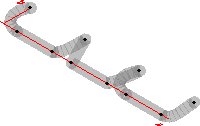        

Three-dimensional versions of bars or arrows can be drawn with one of the specifiers None, Blank, BeginBar3, EndBar3 (or equivalently Bar3), Bars3, BeginArrow3, MidArrow3, EndArrow3 (or equivalently Arrow3), and Arrows3. The predefined three-dimensional arrowhead styles are DefaultHead3, HookHead3, TeXHead3. Versions of the ii-dimensional arrowheads lifted to three-dimensional space and aligned according to the initial viewpoint are likewise divers:

arrowhead3 DefaultHead2(filltype filltype=Fill); arrowhead3 HookHead2(real dir=arrowdir, real barb=arrowbarb,                      filltype filltype=Fill); arrowhead3 TeXHead2;        

An unfilled arrow will be drawn if filltype=NoFill.

Module iii also defines the three-dimensional margins NoMargin3, BeginMargin3, EndMargin3, Margin3, Margins3, BeginPenMargin3, EndPenMargin3, PenMargin3, PenMargins3, BeginDotMargin3, EndDotMargin3, DotMargin3, DotMargins3, Margin3, and TrueMargin3.

Further three-dimensional examples are provided in the files near_earth.asy, conicurv.asy, and (in the animations subdirectory) cube.asy.

Express back up for projected vector graphics (effectively three-dimensional nonrendered PostScript) is bachelor with the setting render=0. This currently only works for piecewise planar surfaces, such every bit those produced by the parametric surface routines in the graph3 module. Surfaces produced by the solids package will as well exist properly rendered if the parameter nslices is sufficiently large.

In the module bsp, hidden surface removal of planar pictures is implemented using a binary space sectionalization and picture clipping. A planar path is first converted to a construction face derived from moving picture. A face may exist given to a two-dimensional cartoon routine in identify of any moving-picture show argument. An array of such faces may so be drawn, removing hidden surfaces:

void add together(picture pic=currentpicture, face[] faces,          projection P=currentprojection);        

Labels may be projected to 2 dimensions, using projection P, onto the plane passing through point O with normal cross(u,v) by multiplying it on the left by the transform

transform transform(triple u, triple v, triple O=O,                     projection P=currentprojection);        

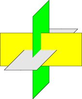
Hither is an example that shows how a binary infinite partition may exist used to describe a PostScript vector prototype of three orthogonal intersecting planes:

size(6cm,0); import bsp;  real u=2.5; real v=1;  currentprojection=oblique;  path3 y=airplane((2u,0,0),(0,2v,0),(-u,-v,0)); path3 l=rotate(90,Z)*rotate(90,Y)*y; path3 one thousand=rotate(xc,X)*rotate(xc,Y)*y;  face[] faces; filldraw(faces.push(y),project(y),yellow); filldraw(faces.push(fifty),project(50),lightgrey); filldraw(faces.push(k),projection(g),light-green);  add(faces);        

---

[ < ]

[ > ]

[ << ]

[ Up ]

[ >> ]

[Meridian]

[Contents]

[Index]

[ ? ]

moraleshisday1968.blogspot.com

Source: https://www.manpagez.com/info/asymptote/asymptote-1.53/asymptote_70.php

Share this post